Proof of termination for Amiko hydras
Introduction
The Amiko hydras post has been the most contentious post I’ve published since I started making content actively. Unlike my other posts, which were quite safe for me as a content creator, this one felt immature, half-hearted, disrespectful even, like a tourist who stopped by a temple to take photos without ever learning about the religion. I thought I would be mocked for naming a salad number, and that this would be a permanent stain on my career. It was a ghost, haunting me, always there, and it would only go away after a proper resolution to give it closure.
If I think about it more, I can tell that’s rubbish, just intrusive thoughts. There’s also impostor syndrome in there, with all the parts that undervalue the work I did. I do not claim now, and did not claim then, that I have contributed as much as the leading mathematicians in ordinal analysis, but I did at least introduce (or at least explicitly describe) a new technique and a new system, so \(AH(4)\) is definitely not a salad number. Even if I never resolved this issue, it would still be alright. Not every post needs to be perfect. People are forgiving, and in time, it just becomes one thing I said in the past, not representing the best of present me. In academia especially, we are forgiving - so long as a contributor can honestly own up to their mistakes, they are forgiven and there is no damage to their record. It’s not a ghost that can haunt me forever.
I also have other good news. I finally have a proof of termination for Amiko hydras, which I hope is correct. A large portion of the work on my part needed to get here wasn’t actually proof writing, but study within the topic. I was already comfortable using the Cantor normal form up to \(\varepsilon_0\), the Veblen normal form up to \(\Gamma_0\), and the Buchholz normal form up to \(\psi_0(\varepsilon_{\Omega_\omega + 1})\). As I see it, there is no point in using the notations between the 2-argument Veblen function and the Buchholz function, including the finitary and transfinite versions of the Veblen function and some other ordinal collapsing functions, as the Buchholz function is simpler than all of those, so you might as well jump up to there.
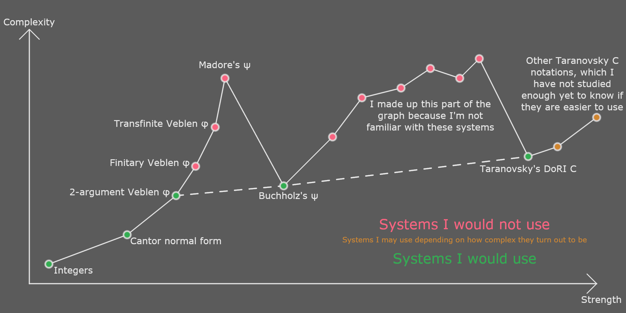
My next major leap was to Taranovsky’s C, specifically the “Degrees of Recursive Inaccessibility” system, which is the weakest one on that page. It took some reading up on background concepts and examining that system until I was comfortable working in it, and it really does not help that that page contains very few examples. Once that was done, I was ready to attempt a proof of termination for Amiko hydras, and that proof itself was actually relatively easy.
Structure of the proof
All ordinals are written in Taranovsky’s DoRI \(C\) normal form.
Let \(\mathbb{H}\) be the set of all hydras. Let \(0_H = (\star:)\). Let \(\chi\) be the limit of Taranovsky’s DoRI \(C\), which is the supremum of all ordinals that can be built using \(C\) and \(0\).
Let \(P\) be “replace all 3-tuples \((a, b, c)\) with \(C(a, b, c)\)”.
Define \(a \lessapprox b\) like so:
1. Definition of termination. \(\forall A \in \mathbb{H}, \pi(A) = (A = 0_H \lor \pi(S(A)))\) Note that \(S\) is nondeterministic due to the free variable \(N\), so there is an implied \(\forall N \in \mathbb{N}\).
In words, \(\pi\) is the predicate “this hydra terminates”. The hydra \(0_H\) is already considered terminated, and any other hydra terminates if after a step it becomes a hydra which terminates.
2. Correspondence from hydras to ordinals. We define a function \(M: \mathbb{H} \to \chi\) with \(M(0_H) = 0\) We define a function \(K\) which is like \(M\) except its output is a tuple, with \(M\) then defined as \(M(A) = P(K(A))\). Let \(\tau(\alpha, m) = (\forall A \in \mathbb{H}, Q(A) \le m \implies ( M(A) = \alpha \implies \pi(A)) )\) We also fix the definition of hydra comparison as \((A \lesseqgtr B) = (M(A) \lesseqgtr M(B))\), which is needed because the original post on the hydras did not explicitly give a comparison algorithm.
In words, \(\tau\) is the predicate “for all hydras which correspond to this ordinal, that hydra terminates”. There may be no such hydras, in which case it is vacuously true.
3. Definition of sub-expression comparison. Define \(a \lessapprox b \iff a \lessapprox^\emptyset b\) Define \(a \lessapprox_=^c b \iff a = b \lor a \lessapprox^c b\) Define \(a \lessapprox^c b \iff b \neq 0 \land (a = 0 \lor a \neq 0 \land (a \lessapprox^{c\cup \{b\}} b[2]\) \(\lor (a[2] \lessapprox_=^{c\cup \{b\}} b[2] \lor a[2] \lessapprox_=^c b) \land (\) \(a[0] \lessapprox^{c\cup \{b\}} b[0] \land (a[1] \lessapprox_=^{c\cup \{b\}} b[1] \lor \exists x \in c\cup \{b\}, a[1]\lessapprox x)\) \(\lor a[0] \lessapprox_=^{c\cup \{b\}} b[0] \land a[1] \lessapprox^{c\cup \{b\}} b[1] )\) \(\lor a[0] \lessapprox_=^{c\cup \{b\}} b[0] \land a[1] \lessapprox_=^{c\cup \{b\}} b[1] \land a[2] \lessapprox^{c\cup \{b\}} b[2] ))\) Note that \(c_0 \subset c_1 \implies (a \lessapprox^{c_0} b \implies a \lessapprox^{c_1} b)\), so it is safe to drop \(c\) in certain contexts, as is done in the proof.
The clause \(\exists x \in c\cup \{b\}, a[1]\lessapprox x\) permits a [1]-term to increase when the [0]-term decreases, but to prevent non-terminating stacking, we still need the [1]-term to be less than something else - to be precise, it must be less than some parent expression.
4. Hydra step always decreases the ordinal or a sub-expression, given that label hydras also decrease. \(\forall A \in (\mathbb{H} - \{0_H\}), (\forall B \in A, K(S(B)) \lessapprox K(B)) \implies K(S(A)) \lessapprox K(A)\) Note that \(S\) is nondeterministic due to the free variable \(N\), so there is an implied \(\forall N \in \mathbb{N}\).
5. Definition of hydra depth. \(Q(A) = \max \{ 0 \} \cup \{ Q(B) + 1 | B \in A \} \)
The depth of \(0_H\) is \(0\), and the depth of all other hydras is \(1\) more than the highest depth of any label.
6. Transfinite induction for termination of hydras with limited depth. We define \(R(m) = (\forall \alpha \in \chi, \tau(\alpha, m))\) Then, \(\tau(0, m) \land (\forall \alpha \in \chi, (\forall \beta \in \alpha, \tau(\beta, m)) \implies \tau(\alpha, m)) \implies R(m)\)
In words, if it holds for \(0\), and if it holds for some \(\alpha\) if it holds for all \(\beta\) below \(\alpha\), then it holds for all ordinals. There is actually nothing wrong with making this claim for all ordinals, but in this context, there is no point going above \(\chi\) anyway, since no hydras map to those large ordinals.
7. Induction on depth for termination of hydras. \((R(0) \land \forall m \in \mathbb{N}, R(m) \implies R(m+1)) \implies \forall m \in \mathbb{N}, R(m)\)
8. If sub-expressions decrease, the ordinal eventually decreases. There is no infinite sequence \(a_0, a_1, \cdots\) for which \(\forall n \in \mathbb{N}, P(a_n) = P(a_{n+1}) \land a_{n+1} \lessapprox a_n\). The formal statement is quite long to write, but it is proven by transfinite induction.
The only non-trivial part of this is step 4. I dedicate some space to defining \(M\), and the rest of the proof is for proving step 4.
Hydra theorem. \(\forall A \in \mathbb{H}, \pi(A)\)
Conjecture. “The strength of Amiko hydras is upper-bounded at \(C(\chi,0)\).” I would be completely sure of this if every step decreased the ordinal. However, I relied on sub-expressions decreasing, which hides additional structure. At the very least, this conjecture does not follow obviously from the main theorem, and it is possible that the additional structure pushes the strength of Amiko hydras above \(C(\chi,0)\).
I must emphasize that, because \(M\) is not necessarily a bijection, \(\chi\) is only an upper bound for the strength of Amiko hydras, and actually the hydras may be weaker. To be precise, for the unique \(\chi\) for which a bijective \(M\) exists, the strength of Amiko hydras is exactly that \(\chi\).
Definition of \(K\)
Let \(A\) be the hydra of discourse.
If \(A = 0_H\), then \(K(A) = 0\). Otherwise:
Let \(\alpha \leftarrow 0\) be an ordinal variable.
For each child \(B\) of \(A\), iterated in descending order, do:
Let \(D\) be \(B\) but with the label changed to \(\star\), which changes it into a root node.
Let \(E\) be the label of \(B\).
Assign \(\alpha \leftarrow (K(E), K(D), \alpha) \).
Then \(K(A) = \alpha\).
Proving the ordinal or a sub-expression always decreases
Definitions
Recall the definition of \(S\):
It is guaranteed if we are reducing \(A\) that it has children. Let \(B\) be the \(A\)’s rightmost child, and let \(C\) be \(B\)’s label.
1. If \(C = (\star:)\): Search for the rightmost leaf of \(A\), but do not enter nodes with labels \( > (\star:)\). Let \(D\) be this rightmost leaf (whose label is guaranteed to be \((\star:)\)).
1.1. If \(D\) has no children: Let \(E\) be the parent of \(D\). Remove \(D\) from \(E\). If \(E\) has a parent, append \(N\) copies of \(E\) as additional children to the parent of \(E\), for some \(N\). \(S(A)\) is the modified \(A\).
1.2. If \(D\) has any children (which are guaranteed to have label \( > (\star:)\)): Traverse up the parents from \(D\) searching for a node \(E\) satisfying \(E <_{> (\star:)} D\) (but do not enter nodes with label \(> (\star:)\)), or if no suitable \(E\) is found, take \(E\) as the last candidate’s parent (or \(A\) if it was reached) but with all children removed except for the rightmost. Let \(D’\) be \(D\) but with the label changed to \(\star\). Let \(E’\) be \(S(D’)\) but without children whose label is \((\star:)\) and with the children of \(E\) whose labels are \((\star:)\) appended as children, and with the label of \(D\). Let \(F = ((\star:):)\). Do this \(N\) times, for some \(N\): “Replace \(F\) with \(E’\) where \(D\) is replaced by \(F\).” Replace \(D\) with \(F\). \(S(A)\) is the modified \(A\).
2. If \(C > (\star:)\): Go right in the tree, looking for the rightmost leaf. If \(C\) has no children the search just ends there.
2.1. If a node \(D\) with label \((\star:)\) is encountered, proceed as in rule 1.
2.2 If we reach a leaf without ever encountering a node with label \((\star:)\): Let \(D\) be this rightmost leaf. Let \(E\) be the label of \(D\). Traverse up the parents from \(D\) searching for a node \(F\) with \(G\) as the label of \(F\) satisfying \(G < E\), which is always guaranteed to exist, because the root always satisfies this. Let \(H = S(E)\). Let \(F’\) be \(F\) but with the label changed to \(H\). Let \(I = ((\star:):)\). Do this \(N\) times, for some \(N\): “Replace \(I\) with \(F’\) where \(D\) is replaced by \(I\)” Replace \(D\) with \(I\). \(S(A)\) is the modified \(A\).
Recall the comparison algorithm for Taranovsky’s DoRI \(C\):
If a and b are maximal in C(a, b, c), then C(a, b, c) < C(d, e, f) iff C(a, b, c) ≤ f or c < C(d, e, f) ∧ (a, b) < (d, e).
Taranovsky, 2020, Section 3.2
This holds for \(C(a, b, c)\) if \(a, b\) are maximal and \(c\) is minimal, which defines the normal form. If both \(C(a, b, c), C(d, e, f)\) are in normal form, then the comparison result is guaranteed to be correct.
Outside of normal form, the comparison algorithm may fail to produce a result, or it may produce a result. Without loss of generality, if in this case it says \(C(a, b, c) < C(d, e, f)\), then all we can actually conclude is \(C(a, b, c) \leq C(d, e, f)\), that is, it may incorrectly determine that 2 different expressions which are the same ordinal are not equal, but a less than or greater than result will never be the opposite of the correct comparison.
I refer to \(C(a, b, c) ≤ f\) as clause 1, \(c < C(d, e, f)\) as clause 2, and \((a, b) < (d, e)\) as clause 3. The definition of \(\lessapprox\) includes analogous clauses, which I will also refer to as clause 1, clause 2, and clause 3.
Rule 1.1
If \(E\) has no parent, it must be the root. In this case, \(M(A) = C(0, 0, \alpha)\) for some ordinal \(\alpha\), and \(M(S(A)) = \alpha\). In this case, the ordinal decreases.
Suppose then that \(E\) does have a parent, \(F\). Let \(F’\) be \(F\) but with the label changed to \(\star\), and define \(E’\) analogously. Note that \(K(F’)\) appears as a sub-expression in \(K(A)\). Let \(G\) be \(F\) after the step, and define \(G’\) analogously. Note that \(K(G’)\) appears as a sub-expression in \(K(S(A))\). In this case, \(M(F’) = C(\alpha, M(E’), \beta) = C(\alpha, C(0, 0, \gamma), \beta)\) for some \(\alpha, \beta, \gamma\), and \(M(G’) = C(\alpha, \gamma, C(\alpha, \gamma, \cdots C(\alpha, \gamma, \beta) \cdots))\) with the number of nestings depending on the chosen \(N\). As long as there are more nestings, clause 1 is false, clause 3 is true, and clause 2 asks us to take off the outermost nesting layer. After doing this \(N\) times, we find \(M(G’) < M(F’) \iff \beta < C(\alpha, C(0, 0, \gamma), \beta)\), which is clearly true. \(F\) may be a sub-expression, so we cannot guarantee \(M(S(A)) < M(A)\), but we are sure that \(K(F’)\) will decrease, so we can say \(K(S(A)) \lessapprox K(A)\).
Rule 2.2
Let \(f_{Z, k}(b) = (a, b, c)\) be a family of functions, where, if \(Y\) is the node reached by repeatedly taking the rightmost child \(k\) times starting with \(Z\), \(c\) is what \(K(Y)\) would be if the rightmost child of \(Y\) was removed, and \(a = K(X)\) where \(X\) is the label of the rightmost child of \(Y\). Let \(f_{Z, m:k} = (f_{Z, m} \circ f_{Z, m+1} \circ \cdots \circ f_{Z, k-3} \circ f_{Z, k-2} \circ f_{Z, k-1})\). Observe \(b_0 \lessapprox b_1 \implies f_{Z, k}(b_0) \lessapprox f_{Z, k}(b_1)\), and additionally \(b_0 \lessapprox b_1 \implies f_{Z, m:k}(b_0) \lessapprox f_{Z, m:k}(b_1)\).
Let \(g(X, Y)\) be the edge distance between nodes \(X, Y\). Observe \(K(A) = f_{A, 0:g(A, D)}(0)\).
Let \(h_{Z, k}(b, a) = (a, b, c)\), with \(c\) defined analogously to how it is defined in \(f\). Let \(h_{Z, m:k} = (f_{Z, m} \circ f_{Z, m+1} \circ \cdots \circ f_{Z, k-3} \circ f_{Z, k-2}) \circ h_{Z, k-1}\), and if \(m=k\), then \(h_{Z, m:k}(b, a) = b\) instead. Observe \(a_0 \lessapprox_=^c a_1 \land (b_0 \lessapprox^c b_1 \lor \exists x \in c\cup \{b_1\},b_0 \lessapprox x)\) \( \implies h_{Z, k}(b_0, a_0) \lessapprox^c f_{Z, k}(b_1, a_1)\). Same applies for \(h_{Z, m:k}\).
Let \(i_{Z, m:k}(b, a_0, a_1, \cdots, a_{j-1}) = h_{Z, m:k}(h_{Z, m:k}(\cdots h_{Z, m:k}(b, a_{j-1}) \cdots, a_1), a_0)\).
Observe \(K(A) = h_{A, 0:g(A, F)}(h_{F, 0:g(F,D)}(0, K(E)), K(G))\). Observe \(K(S(A)) = h_{A, 0:g(A, F)}(0, 0)\) if \(N = 0\), in which case it is obvious that \(K(S(A)) \lessapprox K(A)\). Then, consider \(N > 0\), where \(K(S(A)) = h_{A, 0:g(A, F)}(i_{F, 0:g(F,D)}(0, K(H), K(H), \cdots, K(H), 0), K(G))\), where the innermost argument list uses \(N - 1\) copies of \(K(H)\). Let \(b_1 = 0, a_1 = K(E)\). If we expand the \(i\), the outermost expression uses \(b_0 = 0\) if \(N=1\) and otherwise \(b_0=i_{F, 0:g(F,D)}(0, K(H), K(H), \cdots, K(H), 0)\) with \(N-2\) copies of \(K(H)\), and \(a_0 = K(H)\). Recall \(H = S(E)\). Then \(a_0 = K(H) = K(S(E)) \lessapprox K(E) = a_1\), which we can assume because \(E\) is a label hydra and we are proving this assuming already that label hydras decrease. We also need to show \((b_0 \lessapprox^c b_1 \lor \exists x \in c\cup \{b_1\},b_0 \lessapprox x)\), where \(c\) is the set of parent expressions visited plus \(b_1\) itself, by finding a suitable \(x\). Let \(x\) be the \(K\) of the rightmost child of \(F\). Then \(b_0, x\) look the same until we reach the node corresponding to \(D\). If there are no further layers, then \(b_0 = 0\) and it is obvious we are done. Otherwise, recurse again, choosing the same \(x\). It can be inductively shown then that \((b_0 \lessapprox^c b_1 \lor \exists x \in c\cup \{b_1\},b_0 \lessapprox x)\) for all \(N\). \(a_0 \lessapprox^c a_1 \land b_0 \lessapprox^c b_1\) implies \(i_{F, 0:g(F,D)}(0, K(H), K(H), \cdots, K(H), 0) \lessapprox^c h_{F, 0:g(F,D)}(0, K(E))\), which then implies \(K(S(A)) \lessapprox K(A)\). Thus, in this case, a sub-expression does decrease.
Rule 1.2
Suppose a suitable \(E\) is found. Let \(E^* \) be \(E\) but with label changed to \(\star\). Then, \(K(E^* ) = (a_0, b_0, (a_1, b_1, \cdots (a_{j-1}, b_{j-1}, 0) \cdots ))\) for some \(a, b\). Due to the relative locations, \(K(D)\) must appear as a sub-expression of \(b_0\) (or possibly it is \(b_0\)). Let \(i = \min \{i | i\in j \land 0 \lessapprox a_i \} \cup \{ j \}\). Note that \(\forall k\in i, a_i = 0\). Since a suitable \(E\) was found, and we know \(D\) and \(E\) must both have label \((\star:)\), we can say \((a_i, b_i, (a_{i+1}, b_{i+1}, \cdots (a_{j-1}, b_{j-1}, 0) \cdots )) \lessapprox K(D’)\). Let \(E’^* \) be \(E’\) but with label changed to \(\star\). Let \(D’’\) be \(S(D’)\) but with children with label \((\star:)\) removed. We know \(K(D’’) \lessapprox K(S(D’))\) since removing children causes a sub-expression to decrease, and \(K(S(D’)) \lessapprox K(D’)\) by induction. Then, \(K(D’’) \lessapprox K(D’)\). Observe \(K(E’^* ) = (a_0, b_0, (a_1, b_1, \cdots (a_{i-1}, b_{i-1}, K(D’’)) \cdots )) = (0, b_0, (0, b_1, \cdots (0, b_{i-1}, K(D’’)) \cdots ))\). Observe that the transform “Replace \(F\) with \(E’\) where \(D\) is replaced by \(F\)” corresponds to \(h_{E’, 0:g(E,D)}\). Observe that the iterate corresponds to \(K(F) \mapsto i_{E’, 0:g(E,D)}(K(F), K(G), K(G), \cdots, K(G), 0)\) with \(N-1\) copies of \(K(G)\) where \(G\) is the label of \(D\), however, since we know \(G = (\star:)\), \(K(G) = 0\), and thus the map reduces to simply \(K(F) \mapsto i_{E’, 0:g(E,D)}(K(F), 0, 0, \cdots, 0)\) with \(N\) copies of \(0\). For the original \(F\), if we define \(F^* \) to be \(F\) with label changed to \(\star\), then \(F^* = (\star:)\), and \(K(F^* ) = 0\). Back in \(A\), the subexpression \(K(D’)\) is replaced by \(i_{E’, 0:g(E,D)}(0, 0, 0, \cdots, 0)\) with \(N+1\) copies of \(0\). Our goal is to show \(i_{E’, 0:g(E,D)}(0, 0, 0, \cdots, 0) \lessapprox K(D’)\), which would imply \(K(S(A)) \lessapprox K(A)\). We will do this by showing clause 2 and 3 hold in all cases. For clause 2, we need to take off the outer layer, and check \((0, b_1, \cdots (0, b_{i-1}, K(D’’)) \cdots ) \lessapprox K(D’)\). This happens again at each layer until we reach \(K(D’’) \lessapprox K(D’)\), which we already know to be true. For clause 3, we know \(a[0] = 0 \lessapprox b[0] \neq 0\), and we also need to show \((a[1] \lessapprox_=^{c\cup \{b\}} b[1] \lor \exists x \in c\cup \{b\}, a[1]\lessapprox x)\), where the set \(c\) includes all ancestors of \(K(D’)\). We take the route of showing \(\exists x \in c\cup \{b\}, a[1]\lessapprox x\). Choose the rightmost child of \(E\) here to be \(x\). This mirrors the structure of \(i_{E’, 0:g(E,D)}(0, 0, 0, \cdots, 0)\) until we reach the location where \(D\) would be. There, clause 2 will again hold by the same argument, and clause 3 will allow us to take rightmost child of \(E\) as \(x\) again, while \(a\) now has \(1\) less iterate of the repeated subtree. After moving past all \(N\) iterates, we are left with \(0\) at the leaf being compared to \(K(D’)\), for which it is obvious that \(0 \lessapprox K(D’)\). Thus, in this case, \(K(S(A)) \lessapprox K(A)\).
In another case, suppose no suitable \(E\) was found. In this case, \(E\) is taken as the parent of the last candidate, which may simply be the parent of \(D\) if no nodes were explored, with all children removed except for the rightmost. We can recycle the argument for the previous case, using \(i = j = 1\), and it still works for this case. In this case, \(K(S(A)) \lessapprox K(A)\).
In the last case, suppose \(A\) was reached and still no suitable candidate was found. Then \(A\) is taken as \(E\), with all children removed except for the rightmost. Again, we are able to recycle the previous argument using \(i = j = 1\), so in this case, \(K(S(A)) \lessapprox K(A)\).
Closing comments
I greatly overestimated the difficulty of this task. I am still interested in studying these fields, but I will not ask for a “research opportunity” unless I find something worthy of extensive research.
The actual proof was not hard or obscenely long. Why then, you may wonder, did it take me so long to produce it? It is because I was continually intimidated. In truth, I had all the time in the world and nothing to lose, yet the anxiety persisted. In this landscape, I know where the starting point is, and I know what the goal looks like, but the world is covered in a dense fog. I can look ahead, but never more than a few steps. To ever reach the goal, I needed to try; to break this paralysis; to take some steps. Not every attempt yielded progress. Sometimes I needed to backtrack, and that’s okay. I didn’t get the structure of the proof right the first time, but I would not have derived the other parts, or known I needed a slightly different setup, if I had not made that first attempt. Bit by bit, as I mapped out the path, a working proof emerged.
One important lesson for tackling complex problems like this is that creating structure is helpful. In the geographical analogy, this means identifying landmarks, charting out routes between them, and then putting together the final map. For programmers, this kind of organization is the reason for creating more classes with specific purposes and separating code into multiple files. In this proof, I first introduced some overall structure in the proof, and within the section to prove sub-expressions always decrease, I further divided it by rule and then by cases. There is some complex interdependence, and something like linking in software needs to happen at the very end to produce the final complete proof statement, but so long as I abided by certain rules in logic to avoid issues like circular reasoning, everything would work out.
One more note before I end off my commentary. I’ve long refused to identify with any disability, impairment, or disorder, on the sole basis that I get by fine in life and I’ve never received a formal diagnosis. Not everyone gets by fine though. As a message not for those with a disability but the people they interact with: please be kind to them. If they struggle to do something that seems easy to you, it’s not that they don’t want to, their brain may just be not letting them. Telling them what they need to do or criticizing them does not necessarily enable them to do it.
I know I HAVE to cook, but how do I turn on the stove without the Button?
- Pina, ADHD Alien | Source: WHY CAN YOU DO IT NOW AND NOT EARLIER ? EXECUTIVE DYSFUNCTION THEORY
I’m guilty of doing it in the past, and I almost did it again just now. I commented on my experiences getting here. I don’t expect it to be useful or actionable advice. I did it to tell my story. Thank you for reading.
Appendix - Taranovsky’s DoRI \(C\) examples
To help understand Taranovsky’s DoRI \(C\), I provide many examples against other hopefully more familiar notations. \(\psi\) refers to the extended Buchholz function.
Shorthands I use for Taranovsky’s DoRI \(C\):
- \(C(\alpha, \beta) = C(0, \alpha, \beta)\)
- \(\uparrow \alpha = C(1, 0, \alpha)\) (denoted instead by \(\alpha^+\) on Taranovsky’s page)
- \(\Uparrow \alpha = C(1, 1, \alpha)\)
- \(\Omega = \uparrow 0\) (importantly, not the same as \(\omega_1\), which is what is usually meant by \(\Omega\))
| In other notations | Taranovsky’s DoRI \(C\) |
|---|---|
| \( 0 \) | \( 0 \) |
| \( 1 = \varphi(0, 0) = \psi_0(0) \) | \( C(0, 0) \) |
| \( 2 = \varphi(0, 0) + \varphi(0, 0) = \psi_0(0) + \psi_0(0) \) | \( C(0, 1) = C(0, C(0, 0)) \) |
| \( 3 = \psi_0(0) + \psi_0(0) + \psi_0(0) \) | \( C(0, 2) \) |
| \( \alpha + 1 = \alpha + \psi_0(0) \) | \( C(0, \alpha) \) |
| \( \omega = 1 + 1 + \cdots = \varphi(0, 1) = \varphi(0, \varphi(0, 0)) = \psi_0(1) = \psi_0(\psi_0(0)) \) | \( C(1, 0) = C(C(0, 0), 0) = C(0, C(0, \cdots)) \) |
| \( \omega + 1 \) | \( C(0, C(1, 0)) \) |
| \( \omega + 2 \) | \( C(0, C(0, C(1, 0))) \) |
| \( \omega 2 = \omega + \omega = \omega + 1 + 1 + \cdots = \psi_0(1) + \psi_0(1) \) | \( C(1, C(1, 0)) \) |
| \( \omega 3 \) | \( C(1, C(1, C(1, 0))) \) |
| \( \alpha + \omega \) | \( C(1, \alpha) \) |
| \( \omega^2 = \omega + \omega + \cdots = \varphi(0, 2) = \psi_0(2) \) | \( C(2, 0) = C(1, C(1, \cdots)) \) |
| \( \omega^2 + 1 \) | \( C(0, C(2, 0)) \) |
| \( \omega^2 + \omega \) | \( C(1, C(2, 0)) \) |
| \( \omega^2 2 = \omega^2 + \omega^2 \) | \( C(2, C(2, 0)) \) |
| \( \alpha + \omega^2 \) | \( C(2, \alpha) \) |
| \( \omega^3 = \varphi(0, 3) = \psi_0(3) \) | \( C(3, 0) = C(2, C(2, \cdots)) \) |
| \( \alpha + \omega^3 \) | \( C(3, \alpha) \) |
| \( \omega^n = \varphi(0, n) = \psi_0(n) \) | \( C(n, 0) \) |
| \( \alpha + \omega^n \) | \( C(n, \alpha) \) |
| \( \omega^\omega = \omega^{1 + 1 + \cdots} = \varphi(0, \omega) = \varphi(0, \varphi(0, 1)) = \psi_0(\omega) = \psi_0(\psi_0(1)) = \psi_0(\psi_0(\psi_0(0))) \) | \( C(\omega, 0) = C(C(1, 0), 0) = C(C(0, C(0, \cdots)), 0) \) |
| \( \alpha + \omega^\omega \) | \( C(\omega, \alpha) = C(C(1, 0), \alpha) \) |
| \( \omega^{\omega + 1} = \psi_0(\omega + 1) = \psi_0(\psi_0(1) + 1) \) | \( C(\omega + 1, 0) = C(C(0, C(1, 0)), 0) \) |
| \( \omega^{\omega 2} = \psi_0(\omega 2) = \psi_0(\psi_0(1) 2) \) | \( C(\omega 2, 0) = C(C(1, C(1, 0)), 0) \) |
| \( \omega^{\omega^2} = \psi_0(\omega^2) = \psi_0(\psi_0(2)) \) | \( C(C(2, 0), 0) \) |
| \( \omega^{\omega^\omega} = \varphi(0, \varphi(0, \varphi(0, 1))) = \psi_0(\omega^\omega) = \psi_0(\psi_0(\omega)) = \psi_0(\psi_0(\psi_0(1))) \) | \( C(C(C(1, 0), 0), 0) \) |
| \( \alpha + \omega^\beta = \alpha + \psi_0(\beta), \beta < \varepsilon_0 \) | \( C(\beta, \alpha) \) |
| \( \varepsilon_0 = \omega^{\omega^{\omega^\cdots}} = \varphi(1, 0) = \psi_0(\psi_1(0)) = \psi_0(\psi_0(\psi_0(\cdots))) \) | \( C(\Omega, 0) = C(\uparrow 0, 0) = C(C(1, 0, 0), 0) = C(C(C(\cdots, 0), 0), 0) \) |
| \( \varepsilon_0 + 1 \) | \( C(0, C(\Omega, 0)) \) |
| \( \varepsilon_0 + \omega \) | \( C(1, C(\Omega, 0)) \) |
| \( \varepsilon_0 2 = \varepsilon_0 + \varepsilon_0 = \varepsilon_0 + \omega^{\omega^{\omega^\cdots}} \) | \( C(C(\Omega, 0), C(\Omega, 0)) = C(C(C(C(\cdots, 0), 0), 0), C(\Omega, 0)) \) |
| \( \varepsilon_0 3 \) | \( C(C(\Omega, 0), C(C(\Omega, 0), C(\Omega, 0))) \) |
| \( \omega^{\varepsilon_0 + 1} = \varepsilon_0 \omega = \varepsilon_0 + \varepsilon_0 + \cdots = \varphi(0, \varphi(1, 0) + 1) = \psi_0(\psi_1(0) + 1) \) | \( C(C(0, C(\Omega, 0)), C(\Omega, 0)) = C(C(\Omega, 0), C(C(\Omega, 0), \cdots)) \) |
| \( \omega^{\varepsilon_0 + \omega} = \varepsilon_0 \omega^\omega \) | \( C(C(1, C(\Omega, 0)), C(\Omega, 0)) \) |
| \( \omega^{\omega^{\varepsilon_0 + 1}} = \psi_0(\psi_1(0) + \psi_0(\psi_1(0) + 1)) \) | \( C(C(C(0, C(\Omega, 0)), C(\Omega, 0)), C(\Omega, 0)) \) |
| \( \varepsilon_1 = \varphi(1, 1) = \psi_0(\psi_1(0) 2) \) | \( C(\Omega, C(\Omega, 0)) = C(C(C(\cdots, C(\Omega, 0)), C(\Omega, 0)), C(\Omega, 0)) \) |
| \( \varepsilon_2 = \varphi(1, 2) = \psi_0(\psi_1(0) 3) \) | \( C(\Omega, C(\Omega, C(\Omega, 0))) = C(C(\cdots, C(\Omega, C(\Omega, 0))), C(\Omega, C(\Omega, 0))) \) |
| \( \varepsilon_\omega = \varphi(1, \omega) = \varphi(1, \varphi(0, 1)) = \varepsilon_{1 + 1 + \cdots} = \psi_0(\psi_1(1)) = \psi_0(\psi_1(\psi_0(0))) = \psi_0(\psi_1(0) + \psi_1(0) + \cdots) \) | \( C(\Omega + 1, 0) = C(C(0, \Omega), 0) = C(\Omega, C(\Omega, \cdots)) \) |
| \( \varepsilon_{\omega + 1} = \psi_0(\psi_1(1) + \psi_1(0)) \) | \( C(\Omega, C(C(0, \Omega), 0)) \) |
| \( \varepsilon_{\omega 2} = \psi_0(\psi_1(1) 2) \) | \( C(C(0, \Omega), C(C(0, \Omega), 0)) \) |
| \( \varepsilon_{\omega^2} = \varepsilon_{\omega + \omega + \cdots} = \psi_0(\psi_1(2)) \) | \( C(\Omega + 2, 0) = C(C(0, C(0, \Omega)), 0) = C(C(0, \Omega), C(C(0, \Omega), \cdots)) \) |
| \( \varepsilon_{\omega^n} = \psi_0(\psi_1(n)) \) | \( C(\Omega + n, 0) \) |
| \( \varepsilon_{\omega^\omega} = \psi_0(\psi_1(\psi_0(1))) \) | \( C(\Omega + \omega, 0) = C(C(1, \Omega), 0) \) |
| \( \varepsilon_{\omega^{\omega^\omega}} = \psi_0(\psi_1(\psi_0(\psi_0(1)))) \) | \( C(\Omega + \omega^\omega, 0) = C(C(C(1, 0), \Omega), 0) \) |
| \( \varepsilon_{\varepsilon_0} = \varphi(1, \varphi(1, 0)) = \psi_0(\psi_1(\psi_0(\psi_1(0)))) \) | \( C(\Omega + \varepsilon_0, 0) = C(C(C(\Omega, 0), \Omega), 0) \) |
| \( \varepsilon_{\omega^{\varepsilon_0 + 1}} = \varepsilon_{\varepsilon_0 \omega} = \psi_0(\psi_1(\psi_0(\psi_1(0) + 1))) \) | \( C(\Omega + \varepsilon_0 + 1, 0) = C(C(0, C(C(\Omega, 0), \Omega)), 0) \) |
| \( \varepsilon_{\varepsilon_1} = \varphi(1, \varphi(1, 1)) = \psi_0(\psi_1(\psi_0(\psi_1(0) 2))) \) | \( C(\Omega + \varepsilon_1, 0) = C(C(C(\Omega, C(\Omega, 0)), \Omega), 0) \) |
| \( \varepsilon_{\varepsilon_\omega} = \varphi(1, \varphi(1, \varphi(0, 1))) = \psi_0(\psi_1(\psi_0(\psi_1(1)))) = \psi_0(\psi_1(\psi_0(\psi_1(\psi_0(0))))) \) | \( C(\Omega + \varepsilon_\omega, 0) = C(C(C(C(0, \Omega), 0), \Omega), 0) \) |
| \( \varepsilon_{\varepsilon_{\varepsilon_0}} = \varphi(1, \varphi(1, \varphi(1, 0))) = \psi_0(\psi_1(\psi_0(\psi_1(\psi_0(\psi_1(0)))))) \) | \( C(\Omega + \varepsilon_{\varepsilon_0}, 0) = C(C(C(C(C(\Omega, 0), \Omega), 0), \Omega), 0) \) |
I’ll take a small break here to remind you about how \(C\) is defined.
- C(a, b, c) is the least ordinal e of admissibility degree a that is above c and is not in H(b, e).
- H(b, e) is the least set of ordinals that contains all members of e, and is closed under h, i, j → C(h, i, j) where i < b.
- If an ordinal e is of admissibility degree a, then C(h, i, j) < e whenever h < a and j < e. 0 is of admissibility degree 0.
Taranovsky, 2020, Section 3.1
We won’t need to use \(a > 0\) until larger ordinals, so you can ignore the parts about admissibility degree. In short, \(C(0, b, c)\) is the smallest ordinal above \(c\) which cannot be built from ordinals below it, with the additional restriction that sub-expressions \(C(h, i, j)\) must satisfy \(i < b\).
I think this is where pattern recognition begins to break down and it’s necessary to know the definition. Just from what intuitively makes sense, one would guess \(C(\alpha + 1, 0) = C(\alpha, C(\alpha, \cdots))\) was the regular rule, and that \(C(\Omega, \alpha) = C(C(\cdots, \alpha), \alpha)\) was some special rule. This guess fails at the next example, or if not there, soon after.
| In other notations | Taranovsky’s DoRI \(C\) |
|---|---|
| \( \zeta_0 = \varepsilon_{\varepsilon_{\cdots}} = \varphi(2, 0) = \varphi(1, \varphi(1, \cdots)) = \psi_0(\psi_1(\psi_1(0))) = \psi_0(\psi_1(\psi_0(\psi_1(\cdots)))) \) | \( C(\Omega 2, 0) = C(\Omega + \Omega, 0) = C(C(\Omega, \Omega), 0) = C(C(C(C(\cdots, \Omega), 0), \Omega), 0) \) |
| \( \zeta_0 2 \) | \( C(\zeta_0, \zeta_0) = C(C(C(\Omega, \Omega), 0), C(C(\Omega, \Omega), 0)) \) |
| \( \omega^{\zeta_0 + 1} = \varphi(0, \varphi(2, 0) + 1) = \psi_0(\psi_1(\psi_1(0)) + 1) \) | \( C(\zeta_0 + 1, \zeta_0) = C(C(0, C(C(\Omega, \Omega), 0)), C(C(\Omega, \Omega), 0)) \) |
| \( \varepsilon_{\zeta_0 + 1} = \varphi(1, \varphi(2, 0) + 1) = \psi_0(\psi_1(\psi_1(0)) + \psi_1(0)) \) | \( C(\Omega, \zeta_0) = C(\Omega, C(C(\Omega, \Omega), 0)) \) |
| \( \zeta_1 = \varphi(2, 1) = \psi_0(\psi_1(\psi_1(0)) 2) \) | \( C(\Omega 2, \zeta_0) = C(C(\Omega, \Omega), C(C(\Omega, \Omega), 0)) \) |
| \( \zeta_\omega = \varphi(2, \varphi(0, 1)) = \psi_0(\psi_1(\psi_1(0) + 1)) \) | \( C(\Omega 2 + 1, 0) = C(C(0, C(\Omega, \Omega)), 0) \) |
| \( \zeta_{\zeta_0} = \varphi(2, \varphi(2, 0)) = \psi_0(\psi_1(\psi_1(0) + \psi_0(\psi_1(\psi_1(0))))) \) | \( C(\Omega 2 + \zeta_0, 0) = C(C(C(C(\Omega, \Omega), 0), C(\Omega, \Omega)), 0) \) |
| \( \zeta_{\zeta_\omega} = \varphi(2, \varphi(2, \varphi(0, 1))) = \psi_0(\psi_1(\psi_1(0) + \psi_0(\psi_1(\psi_1(0) + 1)))) \) | \( C(\Omega 2 + \zeta_\omega, 0) = C(C(C(C(0, C(\Omega, \Omega)), 0), C(\Omega, \Omega)), 0) \) |
| \( \varphi(3, 0) = \psi_0(\psi_1(\psi_1(0) 2)) \) | \( C(\Omega 3, 0) = C(\Omega 2 + \Omega, 0) = C(C(\Omega, C(\Omega, \Omega)), 0) \) |
| \( \varphi(3, 1) = \psi_0(\psi_1(\psi_1(0) 2) 2) \) | \( C(C(C(\Omega, C(\Omega, \Omega)), 0), C(C(\Omega, C(\Omega, \Omega)), 0)) \) |
| \( \varphi(3, \varphi(0, 1)) = \psi_0(\psi_1(\psi_1(0) 2 + 1)) \) | \( C(\Omega 3 + 1, 0) = C(C(0, C(\Omega, C(\Omega, \Omega))), 0) \) |
| \( \varphi(3, \varphi(3, 0)) = \psi_0(\psi_1(\psi_1(0) 2 + \psi_0(\psi_1(\psi_1(0) 2)))) \) | \( C(C(C(C(\Omega, C(\Omega, \Omega)), 0), C(\Omega, C(\Omega, \Omega))), 0) \) |
| \( \varphi(3, \varphi(3, \varphi(0, 1))) = \psi_0(\psi_1(\psi_1(0) 2 + \psi_0(\psi_1(\psi_1(0) 2 + 1)))) \) | \( C(C(C(C(0, C(\Omega, C(\Omega, \Omega))), 0), C(\Omega, C(\Omega, \Omega))), 0) \) |
| \( \varphi(4, 0) = \psi_0(\psi_1(\psi_1(0) 3)) \) | \( C(\Omega 4, 0) = C(C(\Omega, C(\Omega, C(\Omega, \Omega))), 0) \) |
| \( \varphi(n + 1, 0) = \psi_0(\psi_1(\psi_1(0) n)) \) | \( C(\Omega (n+1), 0) = C(C(\Omega, \Omega n), 0) \) |
| \( \varphi(\varphi(0, 1), 0) = \psi_0(\psi_1(\psi_1(1))) = \psi_0(\psi_1(\psi_1(\psi_0(0)))) \) | \( C(\omega^{\Omega + 1}, 0) = C(\Omega \omega, 0) = C(C(\Omega + 1, \Omega), 0) = C(C(C(0, \Omega), \Omega), 0) \) |
| \( \varphi(\varphi(0, \varphi(0, 1)), 0) = \psi_0(\psi_1(\psi_1(\psi_0(1)))) = \psi_0(\psi_1(\psi_1(\psi_0(\psi_0(0))))) \) | \( C(C(\Omega + \omega, \Omega), 0) = C(C(C(1, \Omega), \Omega), 0) = C(C(C(C(0, 0), \Omega), \Omega), 0) \) |
| \( \varphi(\varphi(1, 0), 0) = \psi_0(\psi_1(\psi_1(\psi_0(\psi_1(0))))) \) | \( C(C(\Omega + \varepsilon_0, \Omega), 0) = C(C(C(C(\Omega, 0), \Omega), \Omega), 0) \) |
| \( \varphi(\varphi(\varphi(0, 1), 0), 0) = \psi_0(\psi_1(\psi_1(\psi_0(\psi_1(\psi_1(1)))))) \) | \( C(C(C(C(C(C(0, \Omega), \Omega), 0), \Omega), \Omega), 0) \) |
| \( \textbf{Feferman–Schütte ordinal} = \Gamma_0 = \varphi(1, 0, 0) = \psi_0(\psi_1(\psi_1(\psi_1(0)))) \) | \( C(\omega^{\Omega 2}, 0) = C(\Omega^2, 0) = C(C(\Omega 2, \Omega), 0) = C(C(C(\Omega, \Omega), \Omega), 0) \) |
| \( \varphi(\varphi(0, 1), \varphi(1, 0, 0) + 1) = \psi_0(\psi_1(\psi_1(\psi_1(0))) + \psi_1(\psi_1(1))) \) | \( C(\Omega \omega, C(\Omega^2, 0)) = C(C(C(0, \Omega), \Omega), C(C(C(\Omega, \Omega), \Omega), 0)) \) |
| \( \Gamma_1 = \varphi(1, 0, 1) = \psi_0(\psi_1(\psi_1(\psi_1(0))) 2) \) | \( C(\Omega^2, C(\Omega^2, 0)) = C(C(C(\Omega, \Omega), \Omega), C(C(C(\Omega, \Omega), \Omega), 0)) \) |
| \( \Gamma_\omega = \varphi(1, 0, \varphi(0, 1)) = \psi_0(\psi_1(\psi_1(\psi_1(0)) + 1)) \) | \( C(\Omega^2 + 1, 0) = C(C(0, C(C(\Omega, \Omega), \Omega)), 0) \) |
| \( \Gamma_{\Gamma_0} = \varphi(1, 0, \varphi(1, 0, 0)) = \psi_0(\psi_1(\psi_1(\psi_1(0)) + \psi_0(\psi_1(\psi_1(\psi_1(0)))))) \) | \( C(\Omega^2 + \Gamma_0, 0) = C(C(C(C(C(\Omega, \Omega), \Omega), 0), C(C(\Omega, \Omega), \Omega)), 0) \) |
| \( \Gamma_{\Gamma_\omega} = \varphi(1, 0, \varphi(1, 0, \varphi(0, 1))) = \psi_0(\psi_1(\psi_1(\psi_1(0)) + \psi_0(\psi_1(\psi_1(\psi_1(0)) + 1)))) \) | \( C(\Omega^2 + \Gamma_\omega, 0) = C(C(C(C(0, C(C(\Omega, \Omega), \Omega)), 0), C(C(\Omega, \Omega), \Omega)), 0) \) |
| \( \varphi(1, 1, 0) = \psi_0(\psi_1(\psi_1(\psi_1(0)) + \psi_1(0))) \) | \( C(\Omega^2 + \Omega, 0) = C(C(\Omega, C(C(\Omega, \Omega), \Omega)), 0) \) |
| \( \varphi(2, 0, 0) = \psi_0(\psi_1(\psi_1(\psi_1(0)) 2)) \) | \( C(\Omega^2 2, 0) = C(C(C(C(\Omega, \Omega), \Omega), C(C(\Omega, \Omega), \Omega)), 0) \) |
| \( \varphi(\varphi(0, 1), 0, 0) = \psi_0(\psi_1(\psi_1(\psi_1(0) + 1))) \) | \( C(\Omega^2 \omega, 0) = C(\omega^{\Omega 2 + 1}, 0) = C(C(C(0, C(\Omega, \Omega)), \Omega), 0) \) |
| \( \varphi(\varphi(1, 0, 0), 0, 0) = \psi_0(\psi_1(\psi_1(\psi_1(0) + \psi_0(\psi_1(\psi_1(\psi_1(0))))))) \) | \( C(\omega^{\Omega 2 + \varphi(1, 0, 0)}, 0) = C(C(C(C(C(C(\Omega, \Omega), \Omega), 0), C(\Omega, \Omega)), \Omega), 0) \) |
| \( \varphi(\varphi(\varphi(0, 1), 0, 0), 0, 0) = \psi_0(\psi_1(\psi_1(\psi_1(0) + \psi_0(\psi_1(\psi_1(\psi_1(0) + 1)))))) \) | \( C(\omega^{\Omega 2 + \varphi(\varphi(0, 1), 0, 0)}, 0) = C(C(C(C(C(C(0, C(\Omega, \Omega)), \Omega), 0), C(C(\Omega, \Omega), \Omega)), \Omega), 0) \) |
| \( \varphi\begin{bmatrix}1 \\\ 3\end{bmatrix} = \varphi(1, 0, 0, 0) = \psi_0(\psi_1(\psi_1(\psi_1(0) 2))) \) | \( C(\Omega^3, 0) = C(\omega^{\Omega 3}, 0) = C(C(C(\Omega, C(\Omega, \Omega)), \Omega), 0) \) |
| \( \varphi\begin{bmatrix}1 \\\ 4\end{bmatrix} = \varphi(1, 0, 0, 0, 0) = \psi_0(\psi_1(\psi_1(\psi_1(0) 3))) \) | \( C(\Omega^4, 0) = C(\omega^{\Omega 4}, 0) = C(C(C(\Omega, C(\Omega, C(\Omega, \Omega))), \Omega), 0) \) |
| \( \varphi\begin{bmatrix}1 \\\ n + 1\end{bmatrix} = \psi_0(\psi_1(\psi_1(\psi_1(0) n))), n > 0 \) | \( C(\Omega^{n + 1}, 0) = C(C(C(\Omega, \Omega^n), \Omega), 0) \) |
| \( \textbf{Small Veblen ordinal} = \varphi\begin{bmatrix} 1 \\\ \omega \end{bmatrix} = \varphi\begin{bmatrix} 1 \\\ \varphi\begin{bmatrix} 1 \\\ 0 \end{bmatrix} \end{bmatrix} = \psi_0(\psi_1(\psi_1(\psi_1(1)))) \) | \( C(\Omega^\omega, 0) = C(\omega^{\Omega \omega}, 0) = C(\omega^{\omega^{\Omega + 1}}, 0) = C(C(C(C(0, \Omega), \Omega), \Omega), 0) \) |
| \( \varphi\begin{bmatrix} 1 \\\ \varphi\begin{bmatrix} 1 \\\ \varphi\begin{bmatrix} 1 \\\ 0 \end{bmatrix} \end{bmatrix} \end{bmatrix} = \psi_0(\psi_1(\psi_1(\psi_1(\psi_0(\psi_1(\psi_1(\psi_1(1)))))))) \) | \( C(C(C(C(C(C(C(C(0, \Omega), \Omega), \Omega), 0), \Omega), \Omega), \Omega), 0) \) |
| \( \textbf{Large Veblen ordinal} = \psi_0(\psi_1(\psi_1(\psi_1(\psi_1(0))))) \) | \( C(\Omega^\Omega, 0) = C(\omega^{\Omega^2}, 0) = C(\omega^{\omega^{\Omega 2}}, 0) = C(C(C(C(\Omega, \Omega), \Omega), \Omega), 0) \) |
| \( \textbf{Bachmann-Howard ordinal} = \psi_0(\psi_2(0)) \) | \( C(\uparrow\uparrow 0, 0) = C(C(1, 0, C(1, 0, 0)), 0) \) |
I find it remarkable how similar the Buchholz expressions are to the Taranovsky DoRI expressions - if you read Buchholz expressions left to right and Taranovsky right to left, \(\psi_0\) corresponds to \(0\) and \(\psi_1\) corresponds to \(\Omega\). That they are similar would not be too surprising - ordinal collapsing functions, by their nature, tend to have similar looking ladders. Across the zoo of OCFs, including Bachmann’s \(\psi\), Madore’s \(\psi\), Feferman’s \(\theta\), Wilken’s \(\vartheta\), and Weiermann’s \(\vartheta\), if you chart out expressions in each notation that all name the same ordinal, the ladders end up looking similar but will tend to not quite line up, due to differences between the OCFs. What is remarkable to me is that for Buchholz’s \(\psi\) and Taranovsky’s DoRI \(C\), there is a straightforward conversion between them. I am cautious to not speak more on philosophy than is warranted and pollute the serious discussion, but I must say, that the structure stabilizes even while the notation changes (from Buchholz’s \(\psi\) to Taranovsky’s DoRI \(C\)) looks to me to be a good sign we are moving toward the most simple and natural notation.
For the few examples that Taranovsky listed, the corresponding entries in my tables match exactly, so at least to that extent I have verified my derivations are correct.
The final ascent is presented separately and includes \(\varepsilon_0 = \psi_0(\psi_1(0))\) to help make the pattern obvious. I go beyond the normal limit of the Buchholz function using the extended Buchholz function, which doesn’t arbitrarily limit the cardinal index below \(\omega + 1\).
| In other notations | Proof theoretic ordinal of | Taranovsky’s DoRI \(C\) |
|---|---|---|
| \( \varepsilon_0 = \psi_0(\psi_1(0)) \) | \(PA\)1 | \( C(\uparrow 0, 0) = C(C(1, 0, 0), 0) = C(\Omega, 0) \) |
| \( \textbf{Bachmann-Howard ordinal} = \psi_0(\psi_2(0)) \) | \(KP\omega\)2 | \( C(\uparrow\uparrow 0, 0) = C(C(1, 0, C(1, 0, 0)), 0) \) |
| \( \psi_0(\psi_3(0)) \) | \( C(\uparrow\uparrow\uparrow 0, 0) = C(C(1, 0, C(1, 0, C(1, 0, 0))), 0) \) | |
| \( \psi_0(\psi_\omega(0)) \) | \(\Pi_1^1-CA_0\)3 | \( C(\Uparrow 0, 0) = C(C(1, 1, 0), 0) \) |
| \( \textbf{Takeuti-Feferman-Buchholz ordinal} = \psi_0(\psi_{\omega + 1}(0)) \) | \(\Pi_1^1-CA_0+BI\)4 \(\Pi_1^1-CA_0+TI\)3 | \( C(\uparrow\Uparrow 0, 0) = C(C(1, 0, C(1, 1, 0)), 0) \) |
| \( \psi_0(\psi_{\omega 2}(0)) \) | \( C(\Uparrow\Uparrow 0, 0) = C(C(1, 1, C(1, 1, 0)), 0) \) | |
| \( \psi_0(\psi_{\omega^2}(0)) \) | \( C(C(1, 2, 0), 0) \) | |
| \( \psi_0(\psi_{\omega^\omega}(0)) \) | \( C(C(1, C(1, 0), 0), 0) \) | |
| \( \psi_0(\psi_{\omega^{\omega^\omega}}(0)) \) | \( C(C(1, C(C(1, 0), 0), 0), 0) \) | |
| \( \psi_0(\psi_{\varepsilon_0}(0)) = \psi_0(\psi_{\psi_0(\psi_1(0))}(0)) \) | \( C(C(1, C(C(1, 0, 0), 0), 0), 0) \) | |
| \( \psi_0(\psi_{\psi_0(\psi_{\psi_0(\psi_1(0))}(0))}(0)) \) | \( C(C(1, C(C(1, C(C(1, 0, 0), 0), 0), 0), 0), 0) \) | |
| \( \psi_0(\psi_{\psi_1(0)}(0)) \) | \( C(C(1, C(1, 0, 0), 0), 0) \) | |
| \( \psi_0(\psi_{\psi_{\psi_1(0)}(0)}(0)) \) | \( C(C(1, C(1, C(1, 0, 0), 0), 0), 0) \) | |
| \( \psi_0(\Lambda) = \psi_0(\omega_{\omega_{\omega_{\cdots}}}) \) | \(\Pi_1^1-TR_0\)3 | \( C(C(2, 0, 0), 0) \) |
While it is tempting to “continue the pattern” and keep going, it would be quite crude of me to write Buchholz function expressions beyond where even the extended Buchholz function is actually defined. I think this is a good place to stop. Taranovsky’s DoRI \(C\) can go much higher of course - we have matched the strength of Buchholz’s function using only \(C(\alpha, \beta, \gamma)\) with \(\alpha \leq 1\). If you are interested, you can explore that on your own.
-
Kirby, L. and Paris, J. (1982), Accessible Independence Results for Peano Arithmetic. Bulletin of the London Mathematical Society, 14: 285-293. doi:10.1112/blms/14.4.285 ↩
-
Rathjen, M. (1993). Fragments of Kripke-Platek set theory with infinity. In P. Aczel, H. Simmons, & S. Wainer (Eds.), Proof Theory: A selection of papers from the Leeds Proof Theory Programme 1990 (pp. 251-274). Cambridge: Cambridge University Press. doi:10.1017/CBO9780511896262.011 ↩
-
Taranovsky, D. (2020). Ordinal Notation. Retrieved 2020-07-08. ↩ ↩2 ↩3
-
Buchholz, W. (1987), An independence result for (Π11-CA)+BI. Annals of Pure and Applied Logic, 33: 131-155. https://doi.org/10.1016/0168-0072%2887%2990078-9 ↩